Chapter 4 Exploratory Data Analysis
Having retrieved all the necessary data, we now perform some exploratory data analysis on the variables.
Before doing the EDA, we load in some very useful data visualization libraries used by this book Fundementals of Data Visualization - https://serialmentor.com/dataviz/geospatial-data.html
#----load all the libraries needed
# load in libraries
library(tidyverse)
library(scales)
library(lubridate)
library(ggridges)
library(gridExtra)

#----data visualization packages - https://serialmentor.com/dataviz/geospatial-data.html

#install.packages("remotes")
library(remotes)

#devtools::install_github("wilkelab/cowplot")
library(cowplot)

#install.packages("colorspace")
library(colorspace)

#devtools::install_github("clauswilke/colorblindr")
#https://rdrr.io/github/clauswilke/dviz.supp/
#devtools::install_github("clauswilke/dviz.supp")
library(dviz.supp)

#----good bblog post on the formattable package: https://www.littlemissdata.com/blog/prettytables
#install.packages("data.table")
#install.packages("dplyr")
#install.packages("formattable")
#install.packages("tidyr")

library(data.table)
library(dplyr)
library(formattable)
library(tidyr)

#Zivkovic (2019) Great Kaggle Kernel on EDA - https://www.kaggle.com/jaseziv83/a-deep-dive-eda-into-all-variables

options(scipen = 999)
Then, we set up some basic settings from this great Kaggle Kernel by X for data visualisation of exploratory data analysis of variables https://www.kaggle.com/jaseziv83/a-deep-dive-eda-into-all-variables/report
#----set the plotting theme baseline from Zivkovic (2019)
theme_set(theme_minimal() +
            theme(axis.title.x = element_text(size = 15, hjust = 1),
                  axis.title.y = element_text(size = 15),
                  axis.text.x = element_text(size = 12),
                  axis.text.y = element_text(size = 12),
                  panel.grid.major = element_line(linetype = 2),
                  panel.grid.minor = element_line(linetype = 2),
                  plot.margin=unit(c(1,1,-0.5,1),"cm"),
                  plot.title = element_text(size = 18, colour = "grey25", face = "bold"), plot.subtitle = element_text(size = 16, colour = "grey44")))

#----load the colours from Zivkovic (2019)
col_pal <- c("#5EB296", "#4E9EBA", "#F29239", "#C2CE46", "#FF7A7F", "#4D4D4D")
4.1 Airbnb EDA
First we do EDA on the Airbnb data
londonLSOAProfiles_nogeom <- st_set_geometry(londonLSOAProfiles, NULL)## Error in st_set_geometry(londonLSOAProfiles, NULL): could not find function "st_set_geometry"#----use code from blog post to create a formattable table: https://www.littlemissdata.com/blog/prettytables
a1 <- londonLSOAProfiles_nogeom %>%
group_by(LAD11NM) %>%
summarise(
airbnb_freq=mean(airbnb_freq),
airbnb_no_reviews=mean(airbnb_no_reviews),
airbnb_price=mean(airbnb_price),
culture_freq=mean(culture_freq, na.rm=TRUE),
culture_rating=mean(culture_rating, na.rm=TRUE),
culture_av_reviews=mean(culture_av_reviews, na.rm=TRUE)
) %>%
arrange(desc(airbnb_freq)) %>% top_n(n = 11, wt = airbnb_freq)## Error in londonLSOAProfiles_nogeom %>% group_by(LAD11NM) %>% summarise(airbnb_freq = mean(airbnb_freq), : could not find function "%>%"options(digits = 3)
formattable(a1)## Error in formattable(a1): could not find function "formattable"4.1.1 Airbnb freqency distributions
When looking at the distribution of Airbnb listings we see that there are some outliters
#----this distribution function was taken from Zivkovic (2019)
outlier <- round(1.5 * IQR(londonLSOAProfiles$airbnb_freq), 0)

plot1 <- londonLSOAProfiles %>%
          mutate(outlier = ifelse(airbnb_freq > outlier, "Outlier", "Not Outlier")) %>%
          ggplot(aes(x=airbnb_freq)) +
          geom_histogram(alpha = 0.5, fill = "#5EB296", colour = "#4D4D4D") +
          scale_x_continuous(labels = comma) +
          scale_y_continuous(labels = comma) +
          ggtitle("AIRBNB FREQUENCY", subtitle = "Airbnb freqency still skewed even for non-outliers") +
          labs(x= "Airbnb freq per LSOA", y= "Count") +
          facet_wrap(~ outlier, scales = "free")


#----this distribution function was taken from Zivkovic (2019)
outlier <- round(1.5 * IQR(londonLSOAProfiles$airbnb_price), 0)

plot2 <- londonLSOAProfiles %>%
          mutate(outlier = ifelse(airbnb_price > outlier, "Outlier", "Not Outlier")) %>%
          ggplot(aes(x=airbnb_price)) +
          geom_histogram(alpha = 0.5, fill = col_pal[2], colour = "#4D4D4D") +
          scale_x_continuous(labels = comma) +
          scale_y_continuous(labels = comma) +
          ggtitle("AIRBNB PRICE", subtitle = "Airbnb price still skewed even for non-outliers") +
          labs(x= "Airbnb price per LSOA", y= "Count") +
          facet_wrap(~ outlier, scales = "free")


#----this distribution function was taken from Zivkovic (2019)
outlier <- round(1.5 * IQR(londonLSOAProfiles$airbnb_av_reviews), 0)

plot3 <- londonLSOAProfiles %>%
          mutate(outlier = ifelse(airbnb_av_reviews > outlier, "Outlier", "Not Outlier")) %>%
          ggplot(aes(x=airbnb_av_reviews)) +
          geom_histogram(alpha = 0.5, fill = col_pal[3], colour = "#4D4D4D") +
          scale_x_continuous(labels = comma) +
          scale_y_continuous(labels = comma) +
          ggtitle("AIRBNB REVIEWS", subtitle = "Airbnb reviews still skewed even for non-outliers") +
          labs(x= "Airbnb reviews per LSOA", y= "Count") +
          facet_wrap(~ outlier, scales = "free")


g <- grid.arrange(plot1, plot2, plot3, ncol=3)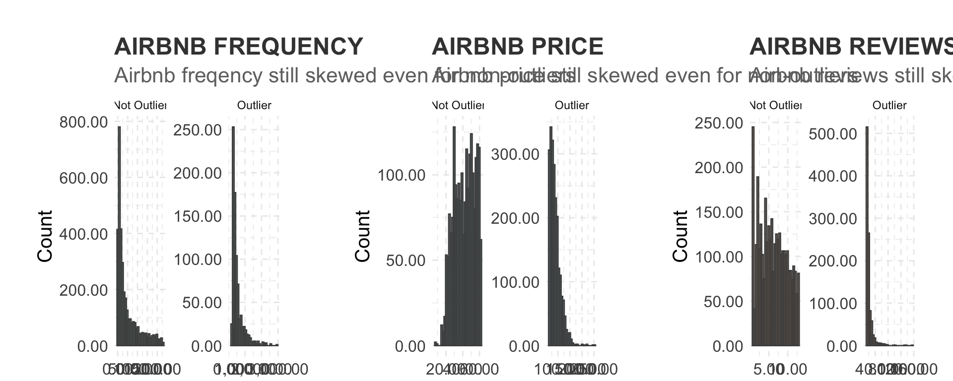
#ggsave("graphs/1.png", plot = g, width = 10, height = 4)4.1.2 Airbnb log freqency distributions
Lets look at the log of Airbnb freqency
#----this log distribution function was taken from Zivkovic (2019)
plot4 <- londonLSOAProfiles %>%
          ggplot(aes(x= log(airbnb_freq))) +
          geom_histogram(alpha = 0.5, fill = "#5EB296", colour = "#4D4D4D") +
          scale_y_continuous(labels = comma) +
          ggtitle("LOG AIRBNB FREQ", subtitle = "The variable looks a lot more workable now") +
          labs(x= "log(Airbnb Freq)", y= "Count")


#----this log distribution function was taken from Zivkovic (2019)
plot5 <- londonLSOAProfiles %>%
          ggplot(aes(x= log(airbnb_price))) +
          geom_histogram(alpha = 0.5, fill = col_pal[2], colour = "#4D4D4D") +
          scale_y_continuous(labels = comma) +
          ggtitle("LOG AIRBNB PRICE", subtitle = "The variable looks a lot more workable now") +
          labs(x= "log(Airbnb price)", y= "Count")


#----this log distribution function was taken from Zivkovic (2019)
plot6 <- londonLSOAProfiles %>%
          ggplot(aes(x= log(airbnb_no_reviews))) +
          geom_histogram(alpha = 0.5, fill = col_pal[3], colour = "#4D4D4D") +
          scale_y_continuous(labels = comma) +
          ggtitle("LOG AIRBNB REVIEWS", subtitle = "The variable looks a lot more workable now") +
          labs(x= "log(Airbnb reviews)", y= "Count")

grid.arrange(plot4, plot5, plot6, ncol=3)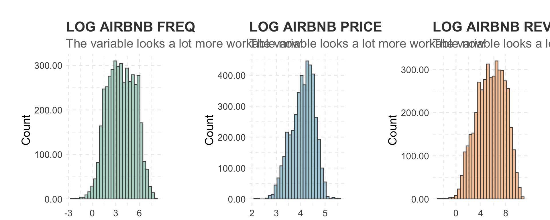
4.1.3 Airbnb Inner vs Outer London
Lets look at Airbnb frequency in Inner vs Outer London
#----this log distribution function was taken from Zivkovic (2019)
plot7 <- londonLSOAProfiles %>%
          ggplot(aes(x= log(airbnb_freq), fill = as.character(InnerOuter))) +
          geom_density(alpha = 0.5, adjust = 2) +
          scale_fill_manual(values = col_pal) +
          ggtitle("THERE ARE MORE LISTINGS IN INNER LONDON", subtitle = "") +
          labs(x= "log(Airbnb Freq)") +
          theme(axis.title.y = element_blank(), legend.position = "top")


#----this log distribution function was taken from Zivkovic (2019)
plot8 <- londonLSOAProfiles %>%
          ggplot(aes(x= log(airbnb_price), fill = as.character(InnerOuter))) +
          geom_density(alpha = 0.5, adjust = 2) +
          scale_fill_manual(values = col_pal) +
          ggtitle("LISTINGS ARE MORE EXPENSIVE IN INNER LONDON", subtitle = "") +
          labs(x= "log(Airbnb Price)") +
          theme(axis.title.y = element_blank(), legend.position = "top")

#----this log distribution function was taken from Zivkovic (2019)
plot9 <- londonLSOAProfiles %>%
          ggplot(aes(x= log(airbnb_no_reviews), fill = as.character(InnerOuter))) +
          geom_density(alpha = 0.5, adjust = 2) +
          scale_fill_manual(values = col_pal) +
          ggtitle("LISTINGS ARE MORE EXPENSIVE IN INNER LONDON", subtitle = "") +
          labs(x= "log(Airbnb Price)") +
          theme(axis.title.y = element_blank(), legend.position = "top")

grid.arrange(plot7, plot8, plot9, ncol=3)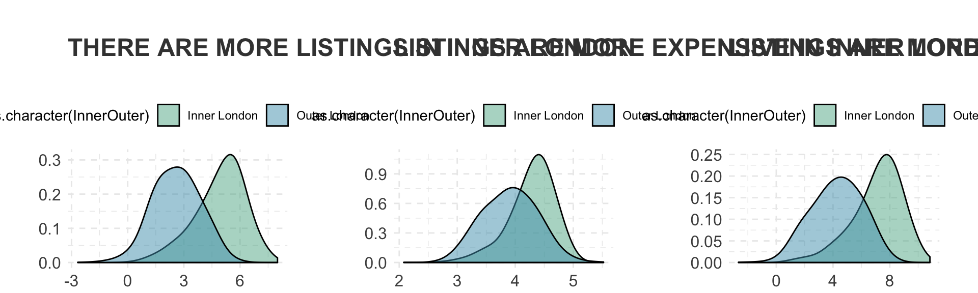
4.2 Cultural infrastructure EDA
Now lets look at cultural infrastructure
4.2.1 Cultural infrastructure frequency distributions
#----this distribution function was taken from Zivkovic (2019)
outlier <- round(1.5 * IQR(londonLSOAProfiles$culture_freq, na.rm = TRUE), 0)

plot10 <- londonLSOAProfiles %>%
            mutate(outlier = ifelse(culture_freq > outlier, "Outlier", "Not Outlier")) %>%
            ggplot(aes(x=culture_freq)) +
            geom_histogram(alpha = 0.5, fill = "#5EB296", colour = "#4D4D4D") +
            scale_x_continuous(labels = comma) +
            scale_y_continuous(labels = comma) +
            ggtitle("CULTURAL INFRASTRUCUTRE IN FREQUENCY", subtitle = "Cultural Infrastructure freqency still skewed even for non-outliers") +
            labs(x= "Cultural Infrastructure freq per LSOA", y= "Count") +
            facet_wrap(~ outlier, scales = "free")


#----this distribution function was taken from Zivkovic (2019)
outlier <- round(1.5 * IQR(londonLSOAProfiles$culture_rating, na.rm = TRUE), 0)

plot11 <- londonLSOAProfiles %>%
            mutate(outlier = ifelse(culture_rating > outlier, "Outlier", "Not Outlier")) %>%
            ggplot(aes(x=culture_rating)) +
            geom_histogram(alpha = 0.5, fill = col_pal[2], colour = "#4D4D4D") +
            scale_x_continuous(labels = comma) +
            scale_y_continuous(labels = comma) +
            ggtitle("CULTURAL INFRASTRUCUTRE Rating", subtitle = "Cultural Infrastructure price still skewed even for non-outliers") +
            labs(x= "Cultural Infrastructure price per LSOA", y= "Count") +
            facet_wrap(~ outlier, scales = "free")


#----this distribution function was taken from Zivkovic (2019)
outlier <- round(1.5 * IQR(londonLSOAProfiles$culture_no_reviews, na.rm = TRUE), 0)

plot12 <- londonLSOAProfiles %>%
            mutate(outlier = ifelse(culture_no_reviews > outlier, "Outlier", "Not Outlier")) %>%
            ggplot(aes(x=culture_no_reviews)) +
            geom_histogram(alpha = 0.5, fill = col_pal[3], colour = "#4D4D4D") +
            scale_x_continuous(labels = comma) +
            scale_y_continuous(labels = comma) +
            ggtitle("CULTURAL INFRASTRUCUTRE REVIEWS", subtitle = "Cultural Infrastructure reviews still skewed even for non-outliers") +
            labs(x= "Cultural Infrastructure reviews per LSOA", y= "Count") +
            facet_wrap(~ outlier, scales = "free")

grid.arrange(plot10, plot11, plot12, ncol=3)
## Warning: Removed 2116 rows containing non-finite values (stat_bin).
## Warning: Removed 2116 rows containing non-finite values (stat_bin).
## Warning: Removed 2116 rows containing non-finite values (stat_bin).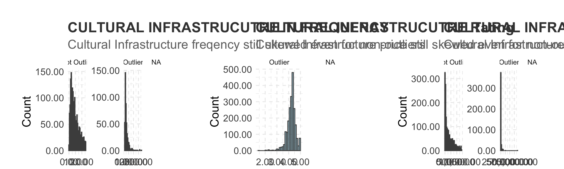
4.2.2 Cultural infrastructure log distibutions
#----this log distribution function was taken from Zivkovic (2019)
plot13 <- londonLSOAProfiles %>%
          ggplot(aes(x= log(culture_freq))) +
          geom_histogram(alpha = 0.5, fill = "#5EB296", colour = "#4D4D4D") +
          scale_y_continuous(labels = comma) +
          ggtitle("LOG CULTURE FREQ", subtitle = "The variable looks a lot more workable now") +
          labs(x= "log(Airbnb Freq)", y= "Count")


#----this log distribution function was taken from Zivkovic (2019)
plot14 <- londonLSOAProfiles %>%
          ggplot(aes(x= culture_rating)) +
          geom_histogram(alpha = 0.5, fill = col_pal[2], colour = "#4D4D4D") +
          scale_y_continuous(labels = comma) +
          ggtitle("LOG CULTURE RATINGS", subtitle = "The variable looks a lot more workable now") +
          labs(x= "log(Airbnb price)", y= "Count")


#----this log distribution function was taken from Zivkovic (2019)
plot15 <- londonLSOAProfiles %>%
          ggplot(aes(x= log(culture_no_reviews))) +
          geom_histogram(alpha = 0.5, fill = col_pal[3], colour = "#4D4D4D") +
          scale_y_continuous(labels = comma) +
          ggtitle("LOG CULTURE REVIEWS", subtitle = "The variable looks a lot more workable now") +
          labs(x= "log(Airbnb reviews)", y= "Count")

grid.arrange(plot13, plot14, plot15, ncol=3)
## Warning: Removed 2116 rows containing non-finite values (stat_bin).
## Warning: Removed 2116 rows containing non-finite values (stat_bin).
## Warning: Removed 2116 rows containing non-finite values (stat_bin).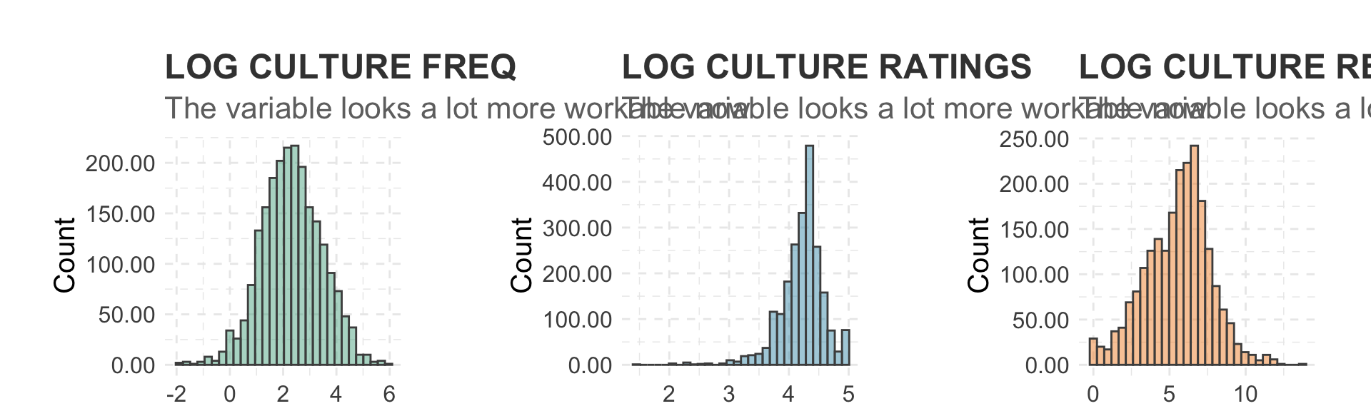
4.2.3 All variables
Freqency distributions
#Use code from MacLachlan & Dennett (2019: chapter 8.2.4) to visualise frequency of dependent variables - https://andrewmaclachlan.github.io/CASA0005repo/online-mapping-descriptive-statistics.html#learning-objectives-1

#----find the column numbers for first and last cultural venue type
which( colnames(londonLSOAProfiles)=="bame_p" )
## [1] 17which( colnames(londonLSOAProfiles)=="housing" )## [1] 28#----check which variables are numeric first
list1 <- as.data.frame(cbind(lapply(londonLSOAProfiles, class)))
list1 <- cbind(list1, seq.int(nrow(list1)))
londonSub <- londonLSOAProfiles[,c(1:2, 17:28)]
#----drop geometry column
londonSub <- st_set_geometry(londonSub, NULL)
library(reshape2)
#----reshape the dataframe with LSOA name and ID as indicies
londonSub <- melt(londonSub, id.vars = 1:2)
attach(londonSub)
#----plot the histograms
hist2 <- ggplot(londonSub, aes(x=value)) +
geom_histogram(aes(y = ..density..)) +
geom_density(colour="red", size=1, adjust=1)
hist2 + facet_wrap(~ variable, scales="free")## Warning: Removed 2 rows containing non-finite values (stat_bin).## Warning: Removed 2 rows containing non-finite values (stat_density).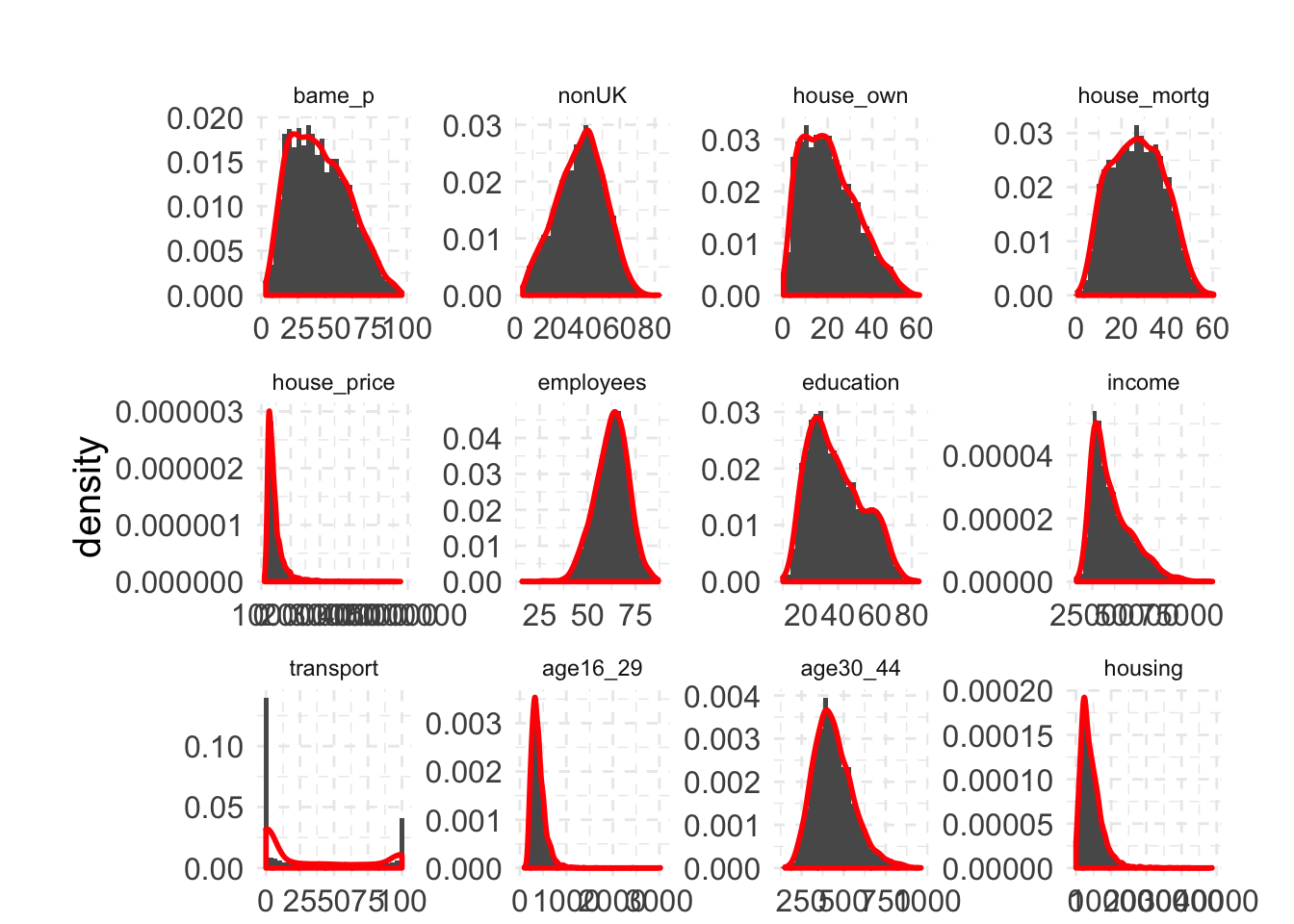
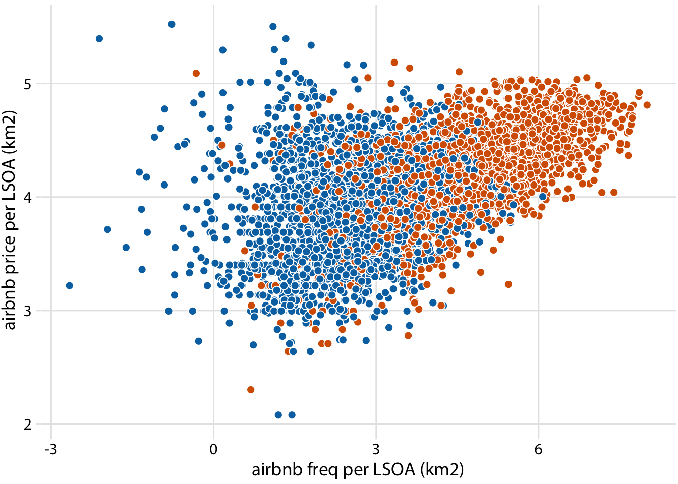
Correlations
#----relationship between dependent variables (Inner vs Outer London)
ggplot(londonLSOAProfiles, aes(log(airbnb_freq), log(airbnb_price), fill = InnerOuter)) +
  geom_point(pch = 21, color = "white", size = 2.5) +
  scale_x_continuous(name = "airbnb freq per LSOA (km2)") +
  scale_y_continuous(name = "airbnb price per LSOA (km2)") +
  scale_fill_manual(
    values = c('Inner London' = "#D55E00", 'Outer London' = "#0072B2"),
    breaks = c("F", "M"),
    labels = c("female birds   ", "male birds"),
    name = NULL,
    guide = guide_legend(
      direction = "horizontal",
      override.aes = list(size = 3)
      )
    ) +
  theme_dviz_grid() +
  theme(
    legend.position = "top",
    legend.justification = "right",
    legend.box.spacing = unit(3.5, "pt"), # distance between legend and plot
    legend.text = element_text(vjust = 0.6),
    legend.spacing.x = unit(2, "pt"),
    legend.background = element_rect(fill = "white", color = NA),
    legend.key.width = unit(10, "pt")
  )
Relationship between culture and airbnb reviews (Inner vs Outer London)
#----relationship between culture and airbnb reviews (Inner vs Outer London)
ggplot(londonLSOAProfiles, aes(log(culture_no_reviews), log(airbnb_no_reviews), fill = InnerOuter)) +
  geom_point(pch = 21, color = "white", size = 2.5) +
  scale_x_continuous(name = "culture_no_reviews PER LSOA (km2)") +
  scale_y_continuous(name = "airbnb_no_reviews LSOA (km2)") +
  scale_fill_manual(
    values = c('Inner London' = "#D55E00", 'Outer London' = "#0072B2"),
    breaks = c("F", "M"),
    labels = c("female birds   ", "male birds"),
    name = NULL,
    guide = guide_legend(
      direction = "horizontal",
      override.aes = list(size = 3)
      )
    ) +
  theme_dviz_grid() +
  theme(
    legend.position = "top",
    legend.justification = "right",
    legend.box.spacing = unit(3.5, "pt"), # distance between legend and plot
    legend.text = element_text(vjust = 0.6),
    legend.spacing.x = unit(2, "pt"),
    legend.background = element_rect(fill = "white", color = NA),
    legend.key.width = unit(10, "pt")
  )
## Warning: Removed 2116 rows containing missing values (geom_point).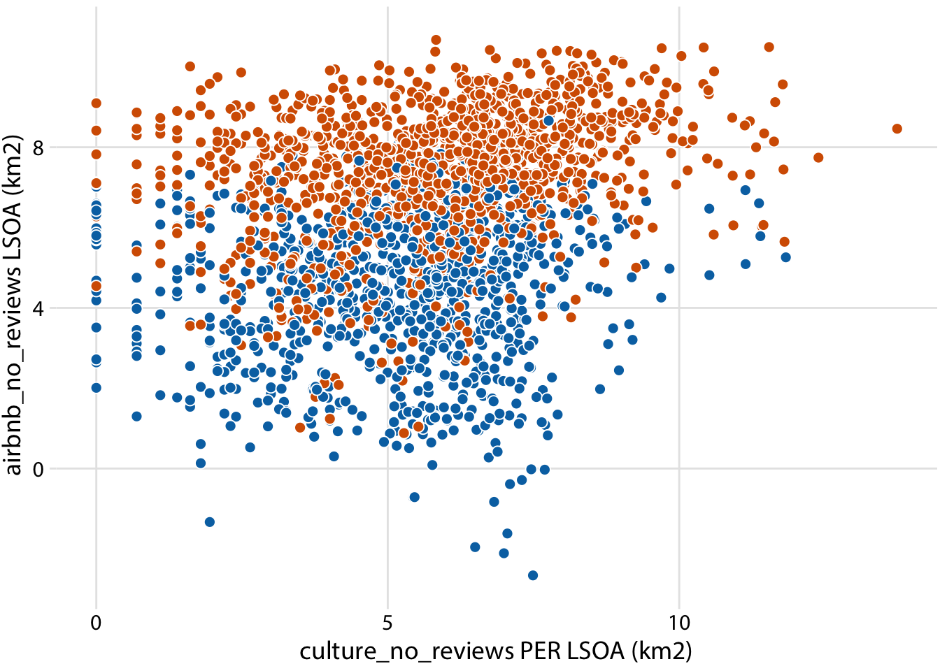
Relationship between culture and airbnb frequency (Inner vs Outer London)
#----relationship between culture and airbnb frequency (Inner vs Outer London)
ggplot(londonLSOAProfiles, aes(log(culture_no_reviews), log(airbnb_freq), fill = InnerOuter)) +
  geom_point(pch = 21, color = "white", size = 2.5) +
  scale_x_continuous(name = "culture_no_reviews PER LSOA (km2)") +
  scale_y_continuous(name = "airbnb_freq LSOA (km2)") +
  scale_fill_manual(
    values = c('Inner London' = "#D55E00", 'Outer London' = "#0072B2"),
    breaks = c("F", "M"),
    labels = c("female birds   ", "male birds"),
    name = NULL,
    guide = guide_legend(
      direction = "horizontal",
      override.aes = list(size = 3)
      )
    ) +
  theme_dviz_grid() +
  theme(
    legend.position = "top",
    legend.justification = "right",
    legend.box.spacing = unit(3.5, "pt"), # distance between legend and plot
    legend.text = element_text(vjust = 0.6),
    legend.spacing.x = unit(2, "pt"),
    legend.background = element_rect(fill = "white", color = NA),
    legend.key.width = unit(10, "pt")
  )
## Warning: Removed 2116 rows containing missing values (geom_point).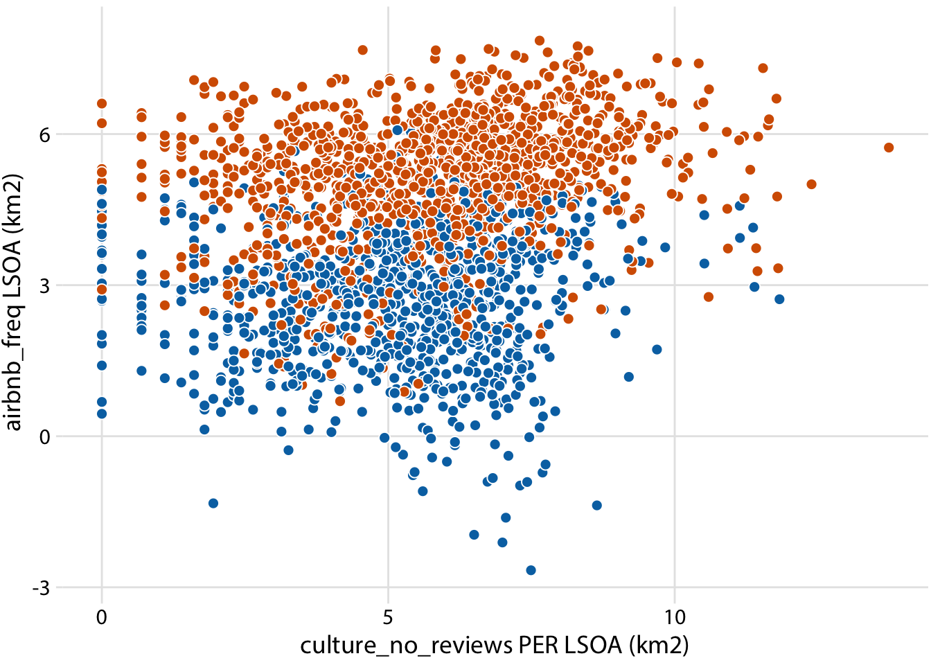
Relationship between culture and airbnb price (Inner vs Outer London)
#----relationship between culture and airbnb price (Inner vs Outer London)
ggplot(londonLSOAProfiles, aes(log(culture_no_reviews), log(airbnb_price), fill = InnerOuter)) +
  geom_point(pch = 21, color = "white", size = 2.5) +
  scale_x_continuous(name = "culture_no_reviews PER LSOA (km2)") +
  scale_y_continuous(name = "airbnb_price LSOA (km2)") +
  scale_fill_manual(
    values = c('Inner London' = "#D55E00", 'Outer London' = "#0072B2"),
    breaks = c("F", "M"),
    labels = c("female birds   ", "male birds"),
    name = NULL,
    guide = guide_legend(
      direction = "horizontal",
      override.aes = list(size = 3)
      )
    ) +
  theme_dviz_grid() +
  theme(
    legend.position = "top",
    legend.justification = "right",
    legend.box.spacing = unit(3.5, "pt"), # distance between legend and plot
    legend.text = element_text(vjust = 0.6),
    legend.spacing.x = unit(2, "pt"),
    legend.background = element_rect(fill = "white", color = NA),
    legend.key.width = unit(10, "pt")
  )
## Warning: Removed 2116 rows containing missing values (geom_point).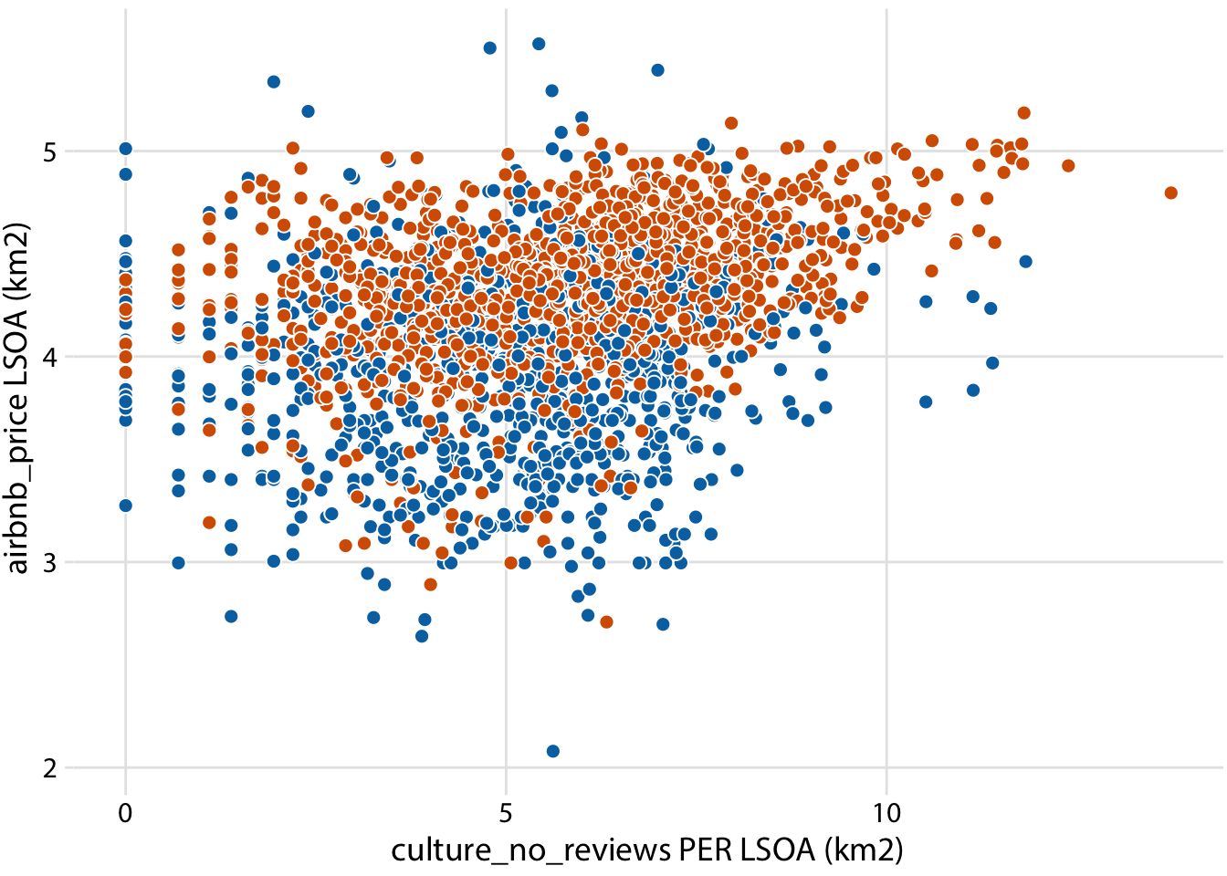
ggplot(londonLSOAProfiles, aes(log(culture_no_reviews), log(house_price), fill = InnerOuter)) +
  geom_point(pch = 21, color = "white", size = 2.5) +
  scale_x_continuous(name = "culture_no_reviews PER LSOA (km2)") +
  scale_y_continuous(name = "house_price LSOA (km2)") +
  scale_fill_manual(
    values = c('Inner London' = "#D55E00", 'Outer London' = "#0072B2"),
    breaks = c("F", "M"),
    labels = c("female birds   ", "male birds"),
    name = NULL,
    guide = guide_legend(
      direction = "horizontal",
      override.aes = list(size = 3)
      )
    ) +
  theme_dviz_grid() +
  theme(
    #legend.position = c(1, 0.01),
    #legend.justification = c(1, 0),
    legend.position = "top",
    legend.justification = "right",
    legend.box.spacing = unit(3.5, "pt"), # distance between legend and plot
    legend.text = element_text(vjust = 0.6),
    legend.spacing.x = unit(2, "pt"),
    legend.background = element_rect(fill = "white", color = NA),
    legend.key.width = unit(10, "pt")
  )
## Warning: Removed 2118 rows containing missing values (geom_point).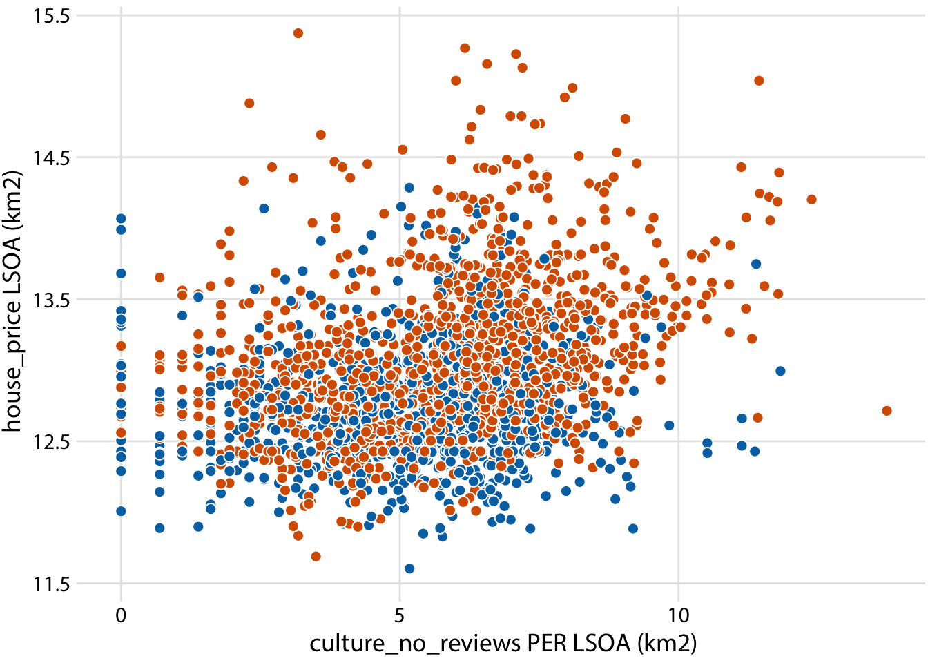
ggplot(londonLSOAProfiles, aes(log(culture_freq), log(house_price), fill = InnerOuter)) +
  geom_point(pch = 21, color = "white", size = 2.5) +
  scale_x_continuous(name = "culture_freq PER LSOA (km2)") +
  scale_y_continuous(name = "house_price LSOA (km2)") +
  scale_fill_manual(
    values = c('Inner London' = "#D55E00", 'Outer London' = "#0072B2"),
    breaks = c("F", "M"),
    labels = c("female birds   ", "male birds"),
    name = NULL,
    guide = guide_legend(
      direction = "horizontal",
      override.aes = list(size = 3)
      )
    ) +
  theme_dviz_grid() +
  theme(
    #legend.position = c(1, 0.01),
    #legend.justification = c(1, 0),
    legend.position = "top",
    legend.justification = "right",
    legend.box.spacing = unit(3.5, "pt"), # distance between legend and plot
    legend.text = element_text(vjust = 0.6),
    legend.spacing.x = unit(2, "pt"),
    legend.background = element_rect(fill = "white", color = NA),
    legend.key.width = unit(10, "pt")
  )
## Warning: Removed 2118 rows containing missing values (geom_point).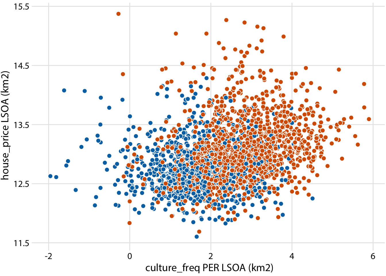
ggplot(londonLSOAProfiles, aes(culture_rating, log(house_price), fill = InnerOuter)) +
  geom_point(pch = 21, color = "white", size = 2.5) +
  scale_x_continuous(name = "culture_rating PER LSOA (km2)") +
  scale_y_continuous(name = "house_price LSOA (km2)") +
  scale_fill_manual(
    values = c('Inner London' = "#D55E00", 'Outer London' = "#0072B2"),
    breaks = c("F", "M"),
    labels = c("female birds   ", "male birds"),
    name = NULL,
    guide = guide_legend(
      direction = "horizontal",
      override.aes = list(size = 3)
      )
    ) +
  theme_dviz_grid() +
  theme(
    #legend.position = c(1, 0.01),
    #legend.justification = c(1, 0),
    legend.position = "top",
    legend.justification = "right",
    legend.box.spacing = unit(3.5, "pt"), # distance between legend and plot
    legend.text = element_text(vjust = 0.6),
    legend.spacing.x = unit(2, "pt"),
    legend.background = element_rect(fill = "white", color = NA),
    legend.key.width = unit(10, "pt")
  )
## Warning: Removed 2118 rows containing missing values (geom_point).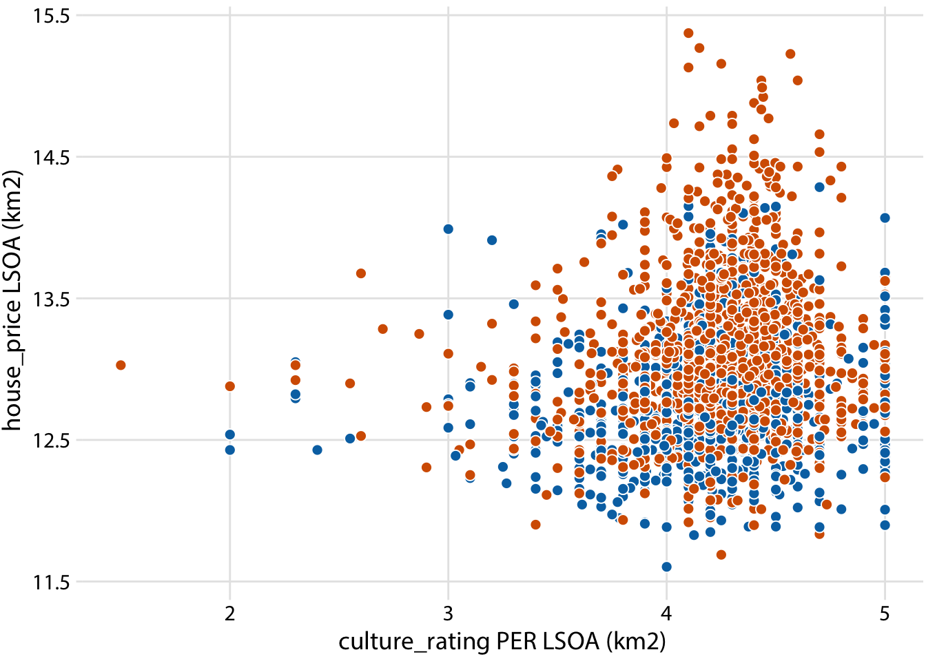
#select some variables from the data file
myvars <- c("airbnb_price",
"airbnb_freq",
'young_p',
'pop_density',
'bame_p',
'nonUK',
'education',
'employees',
'income',
'housing',
'house_own',
'house_mortg',
'house_price',
'transport',
"culture_freq")
#Extracting data.frame from simple features object in R - https://gis.stackexchange.com/questions/224915/extracting-data-frame-from-simple-features-object-in-r
x <- londonLSOAProfiles[myvars]
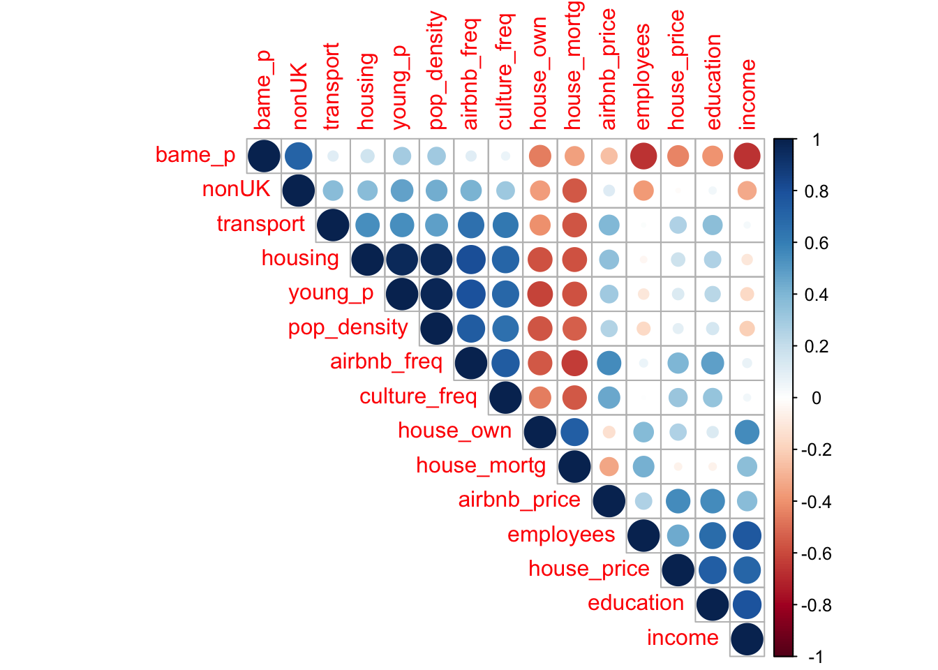
st_geometry(x) <- NULL
class(x)## [1] "data.frame"#check their correlations are OK
#install.packages("Hmisc")
#http://www.sthda.com/english/wiki/correlation-matrix-a-quick-start-guide-to-analyze-format-and-visualize-a-correlation-matrix-using-r-software
library("Hmisc")
cormat <- rcorr(as.matrix(x), type = c("spearman"))
library(corrplot)
# Insignificant correlations are leaved blank
corrplot(cormat$r, type="upper", order="hclust",
p.mat = cormat$S, sig.level = 0.1, insig = "blank")